



Hybrid Machine Learning-Weibull for Remaining Useful Life Prediction
Bridging Statistical Reliability Models and Edge-Cloud Telemetry for Dynamic Remaining Useful Life (RUL) Estimation.
 Go to GitHub Repository
Technologies & Tools
Skills & Competencies
The Problem Statement
Traditional Predictive Maintenance (PdM) systems rely heavily on static, historical averages for survival modeling. These rigid, time-invariant parameters fail to account for dynamic, real-time operational stressors like varying payloads, sudden throttle adjustments, and erratic environmental temperatures, leading to suboptimal or inaccurate Remaining Useful Life (RUL) predictions.
The Core Innovation
This framework transforms the Weibull scale parameter (\(\lambda\)) from a static characteristic lifetime into a dynamic, covariate-driven target for machine learning regression models. By coupling statistical reliability theory directly with advanced regressors, the system produces a percentage-based failure probability curve that adapts continuously to telemetry stressors.
Mathematical Foundation & Interactive Explorer
The Weibull distribution is parameterized by two essential parameters that define failure mechanics:
-
Shape Parameter (\(k\)): Defines the failure nature over time.
- \(k < 1\): Infant mortality (decreasing failure rate).
- \(k = 1\): Random failures (constant failure rate; reduces to Exponential Distribution).
- \(k > 1\): Wear-out phase (increasing failure rate; typical in mechanical structures).
- Scale Parameter (\(\lambda\)): Denotes the characteristic life. It represents the point in time at which approximately 63.2% of all test components are expected to fail, regardless of the shape parameter \(k\).
The Probability Density Function (PDF) and Cumulative Distribution Function (CDF) are represented as:
PDF: \[f(t; k, \lambda) = \frac{k}{\lambda} \left( \frac{t}{\lambda} \right)^{k-1} e^{-\left(\frac{t}{\lambda}\right)^k}\]
CDF: \[F(t; k, \lambda) = 1 - e^{-\left(\frac{t}{\lambda}\right)^k}\]
The Novelty: Custom Weibull Error Metrics
Traditional metrics (like RMSE and MAE) evaluate prediction error based on absolute distance between point targets. This is insufficient for survivability profiles where we want to evaluate the matching of the probability density curves. Thus, custom Weibull error metrics were developed to isolate the mathematical alignment of estimated curves.
These metrics calculate the area between the continuous predicted Weibull Cumulative Distribution Function (CDF) and the actual step function of the failure event (which transitions from 0 to 1 at the actual failure time \(t_{act}\)).
Mean Weibull Error (MWE)
Mean Weibull Error evaluates the cumulative distance of the predicted scale parameter \(\lambda\) from the actual failure point, effectively mapping standard deviation equivalents over survival profiles.
def weibull_error_dataset(x_test, x_pred, k):
    sum_error = 0
    for x, lmbda in zip(x_test, x_pred):
        sum_error += weibull_error(x, lmbda, k)
    return sum_error / len(x_test)
Mean Quadratic Weibull Error (MQWE)
MQWE enforces high quadratic penalties for extreme anomalies, evaluating the general reliability curve deviations on outliers. It is critical for safety-critical hardware where catastrophic failures must be avoided.
def quadratic_weibull_error_dataset(x_test, x_pred, k):
    sum_error = 0
    for x, lmbda in zip(x_test, x_pred):
        sum_error += weibull_error(x, lmbda, k) ** 2
    return sum_error / len(x_test)
Mean Directional Errors (MRWE & MLWE)
Mean Left Weibull Error (MLWE) and Mean Right Weibull Error (MRWE) are used to isolate whether a model is aggressively over-predicting or under-predicting the failure threshold.
def left_weibull_error(x, lmbda, k):
    lmbda = lmbda if lmbda > 0 else 1e-12
    s = 1.0 / k
    z = (x / lmbda) ** k
    gamma_s = gamma(s)
    l_gamma = gammaincc(s, z) * gamma_s
    l_gamma_0 = gammaincc(s, 0) * gamma_s
    return x + (lmbda * l_gamma / k) - (lmbda * l_gamma_0 / k)

def right_weibull_error(x, lmbda, k):
    lmbda = lmbda if lmbda > 0 else 1e-12
    s = 1.0 / k
    z = (x / lmbda) ** k
    gamma_s = gamma(s)
    l_gamma = gammaincc(s, z) * gamma_s
    return lmbda * l_gamma / k
Scipy Integration & Core Math
Calculations use Scipy's special incomplete gamma functions to evaluate the probability densities dynamically on every telemetry step.
from scipy.special import gamma, gammaincc

def weibull_error(x, lmbda, k):
    lmbda = lmbda if lmbda > 0 else 1e-12
    s = 1.0 / k
    z = (x / lmbda) ** k
    gamma_s = gamma(s)
    l_gamma = gammaincc(s, z) * gamma_s
    l_gamma_0 = gammaincc(s, 0) * gamma_s
    return x + (2 * lmbda * l_gamma / k) - (lmbda * l_gamma_0 / k)
Interactive Weibull Error Explorer
Adjust the telemetry failure target and the model's predicted parameters to see how errors are distributed.
Applied Project I: Edge-Cloud Tire Degradation System
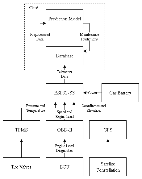
This project maps real-time telemetry captured via a custom gateway board on a moving vehicle into predictive tyre failure curves. The workflow follows a clean vertical architecture:
IoT Edge Gateway & Telemetry
Data is captured on the vehicle using an ESP32-S3 microcontroller acting as an edge gateway. Live sensor packages collect TPMS data (tyre pressures and temperatures), OBD-II diagnostics (engine load and current speeds), and spatial GPS logs to track high-accuracy mileage.
Real-World Data Engineering & Preprocessing
Real-world telemetry gathered from IoT microcontrollers is highly asynchronous, noisy, and prone to packet drops. A comprehensive mathematical and data preprocessing pipeline was engineered to clean, smooth, and transform the raw sensor data:
-
1. Spatial Outlier Detection (IQR Bounds):
Erratic coordinate jumps due to temporary GPS signal loss or multipath propagation are detected and filtered using the Interquartile Range (IQR) method:
\[IQR = Q_3 - Q_1 \quad \implies \quad \text{Valid Range} = [Q_1 - 1.5 \times IQR, \; Q_3 + 1.5 \times IQR]\]
def delete_outlier_gps(df): df_copy = df.copy() for col_name in ['latitude', 'longitude']: Q1 = df.loc[:, col_name].quantile(0.25) Q3 = df.loc[:, col_name].quantile(0.75) IQR = Q3 - Q1 lower_bound = Q1 - 1.5 * IQR upper_bound = Q3 + 1.5 * IQR df_copy = df_copy[(df_copy[col_name] >= lower_bound) & (df_copy[col_name] <= upper_bound)] df_copy.reset_index(drop=True, inplace=True) return df_copy -
2. Geodesic Distance Tracking (Haversine Formula):
Spherical distance (meters) between consecutive spatial coordinates is computed using the Haversine formula (Earth's radius \(R \approx 6,371,000\text{ m}\)):
\[a = \sin^2\left(\frac{\Delta\phi}{2}\right) + \cos(\phi_1)\cos(\phi_2)\sin^2\left(\frac{\Delta\theta}{2}\right)\] \[d = 2R \cdot \operatorname{arctan2}\left(\sqrt{a}, \sqrt{1-a}\right)\]Packets with anomalous jumps (\(d_i > 1000\text{ m}\)) are discarded. The cumulative distance traveled is calculated using a rolling prefix sum (\(\sum d_i\)).
def change_to_distance(df): df_copy = df.copy() df_copy.reset_index(drop=True, inplace=True) for i in range(1, len(df_copy)): lat1, lon1 = df_copy.loc[i-1, 'latitude'], df_copy.loc[i-1, 'longitude'] lat2, lon2 = df_copy.loc[i, 'latitude'], df_copy.loc[i, 'longitude'] distance_km = haversine((lat1, lon1), (lat2, lon2), unit=Unit.METERS) df_copy.loc[i, 'distance_traveled_m'] = distance_km df_copy.at[0, 'distance_traveled_m'] = 0 df_copy['sum_distance_traveled_m'] = df_copy['distance_traveled_m'].cumsum() return df_copy -
3. Telemetry Smearing & Packet Drop Compensation:
Loss of sensor telemetry packets (which register as 0 values in TPMS outputs) are converted to
NaNand then filled sequentially. We apply a backward fill (bfill) to resolve initial zero readings, followed by a forward fill (ffill) to propagate the last known telemetry:\[\mathbf{x}_{\text{smeared}} = \operatorname{ffill}\Big(\operatorname{bfill}\big(\{x_i \mid x_i \neq 0, \text{ else } \text{NaN}\}\big)\Big)\]def smear_temp_pressure(df): df_copy = df.copy() for col_prefix in ['fl', 'fr', 'rl', 'rr']: for suffix in ['temp', 'pressure']: col_name = f'{col_prefix}_{suffix}' df_copy.loc[df_copy[col_name] == 0, col_name] = np.nan df_copy[col_name] = df_copy[col_name].bfill().ffill() return df_copy -
4. Vertical Load Stressor (Elevation Delta):
Vertical elevation adjustments between snapshots are computed to capture grade changes and additional mechanical loading on tires:
\[\Delta E_i = H_i - H_{i-1} \quad (H = \text{altitude in meters})\]
def change_to_elevation(df):
    df_copy = df.copy()
    df_copy.reset_index(drop=True, inplace=True)
    for i in range(1, len(df_copy)):
        alt_1 = df_copy.loc[i-1, 'altitude']
        alt_2 = df_copy.loc[i, 'altitude']
        df_copy.loc[i, 'elevation_traveled_m'] = alt_2 - alt_1
    df_copy.at[0, 'elevation_traveled_m'] = 0
    return df_copy
Model Optimization & Deployment
Models are trained to predict the dynamic \(\lambda\) parameter. LightGBM achieved a Mean Absolute Percentage Error (MAPE) of 0.0025 and Mean Absolute Scaled Error (MASE) of 0.2168. Models are then serialized for cloud server deployment.
from sklearn.model_selection import GridSearchCV
import lightgbm as lgb
import pickle

lightgbm_hyperparam = {
    'num_leaves': [20, 31, 50, 80],
    'min_child_samples': [20, 50, 100],
    'max_depth': [-1, 5, 8],
    'force_col_wise': [True]
}
lightgbm_grid = GridSearchCV(estimator=lgb.LGBMRegressor(), param_grid=lightgbm_hyperparam, cv=3)
lightgbm_grid.fit(X_train, y_train)
with open('lightgbm_grid.pkl', 'wb') as f:
    pickle.dump(lightgbm_grid.best_estimator_, f)
System Demonstration Video
Watch the real-time telemetry streaming from the ESP32-S3 edge gateway to the cloud dashboard and dynamic predictive degradation curve updates in action:
Model Evaluation & Performance Metrics
The models were rigorously evaluated on the tire telemetry dataset using standard regression metrics along with the custom Weibull-specific metrics to measure survival curve alignment:
| Model | MAPE | SMAPE | MASE | MWE | MQWE | MLWE | MRWE |
|---|---|---|---|---|---|---|---|
| LightGBM (Iterative) | 0.0025 (0.25%) | 0.0018 (0.18%) | 0.2169 | 23,603.94 | 7.57e+08 | 13,909.91 | 9,694.03 |
| XGBoost (Iterative) | 0.0038 (0.38%) | 0.0031 (0.31%) | 0.3112 | 23,609.09 | 7.57e+08 | 13,901.89 | 9,707.20 |
| AFT OLS (Iterative) | 0.1426 (14.26%) | 0.1419 (14.19%) | 18.8291 | 24,918.84 | 9.06e+08 | 13,762.53 | 11,156.32 |
| No Covariate (Baseline) | 0.7508 (75.08%) | 0.5557 (55.57%) | 67.0644 | 31,147.55 | 1.09e+09 | 18,227.45 | 12,920.10 |
Conclusions & Key Insights
Traditional reliability schedules (represented by the No Covariate baseline) perform poorly under real-world variables, exhibiting a high MAPE of 75.08%. Modeling the scale parameter using Accelerating Failure Time (AFT) OLS improves estimates to a MAPE of 14.26%, but is limited by the linear assumptions of traditional regression. The machine learning regressors (XGBoost and LightGBM) yield a dramatic increase in performance by successfully learning non-linear stress patterns. LightGBM delivers the most accurate survival prediction, achieving a MAPE of 0.25% and a MASE of 0.2169, which confirms that data-driven machine learning models can dynamically adjust Weibull parameters to reflect real-time operational wear.
Applied Project II: Aircraft Engine Simulation (C-MAPSS)
This benchmark study evaluates the NASA Turbofan Engine Degradation Simulation Dataset (C-MAPSS) to predict the Remaining Useful Life of high-pressure turbine units. Handling 21 disparate sensor measurements over multi-fault conditions (FD003 dataset) reveals critical data-handling findings:
Preprocessing Pipelines
Comparative analysis shows preprocessing design dictates accuracy more than the final regressor choice. A grid of 12 preprocessing combinations (Moving Average, EWMA, Wavelet x Scalers) was instantiated.
from sklearn.preprocessing import StandardScaler, MinMaxScaler
denoising = ['ma', 'ewma', 'wavelet', 'none']
scalers = [StandardScaler(), MinMaxScaler()]
Wavelet Denoising Failure
Wavelet thresholding severely degraded model performance. Denoising stripped critical high-frequency transient signals representing early blade cracking.
import pywt
def wavelet_denoise(signal):
    coeffs = pywt.wavedec(signal, 'db4', level=1)
    uthresh = np.std(coeffs[-1]) * np.sqrt(2 * np.log(len(signal)))
    coeffs[1:] = [pywt.threshold(c, value=uthresh) for c in coeffs[1:]]
    return pywt.waverec(coeffs, 'db4')
Simple Moving Average
Simple Moving Average (SMA) or No Denoising yielded the optimal baselines. These preserved the wear-out trends without flattening the operational stressors.
def apply_sma(df, sensor_cols, window=5):
    for unit_id in df['unit_number'].unique():
        for col in sensor_cols:
            mask = df['unit_number'] == unit_id
            df.loc(mask, col) = df[mask][col].rolling(window).mean()
    return df
XGBoost Robustness
XGBoost proved to be the most robust architecture against the complex multi-fault dataset, resisting overfitting on transient sensor failures.
import xgboost as xgb
xgb_regressor = xgb.XGBRegressor(
    n_estimators=500,
    max_depth=5,
    learning_rate=0.05
)
xgb_regressor.fit(X_train_fd003, y_train_fd003)
The Mathematical Hazard Bridge
The hazard function establishes the dynamic wear-out baseline by calculating failure rate at time x given shape (k) and scale (lambda) parameters:
# Dynamic wear-out hazard function that bridges statistical theory and ML predictions
def hazard(x, k=4.359886822599401, lamb=236.76593258114204):
    return (k / lamb) * ((x / lamb) ** (k - 1))
Model Evaluation & Performance Metrics
The performance of various models evaluated on the turbofan engine dataset (FD001) under multiple preprocessing configurations highlights the strength of the hybrid framework:
| Model | MAE | RMSE | R² Score | MWE (Weibull Error) | MQWE | MLWE | MRWE |
|---|---|---|---|---|---|---|---|
| LightGBM (Linear Time) | 25.44 | 34.21 | 0.3222 | 27.16 | 1,058.44 | 9.07 | 18.09 |
| XGBoost (Linear Time) | 26.59 | 35.08 | 0.2875 | 27.86 | 1,100.96 | 9.03 | 18.83 |
| Random Forest (Linear Time) | 26.62 | 34.83 | 0.2976 | 28.20 | 1,107.17 | 9.78 | 18.43 |
| SVM (Linear Time) | 29.74 | 36.85 | 0.2136 | 30.56 | 1,256.38 | 11.90 | 18.67 |
| Linear Regression | 35.43 | 41.31 | 0.0118 | 34.37 | 1,448.33 | 9.56 | 24.82 |
| AFT OLS (Baseline) | 36.17 | 48.64 | 0.9726 | 44.09 | 2,427.67 | 10.68 | 33.40 |
| No Covariate (Baseline) | 38.50 | 50.53 | 0.9704 | 43.18 | 2,279.94 | 10.83 | 32.35 |
Conclusions & Key Insights
As detailed in the ETASR and ICICyTA papers, the study proves that a covariate-driven Weibull scale parameter regression outperforms static modeling. Simple linear regression and traditional survival modeling fail to capture the degradation kinetics under multi-fault flying environments. LightGBM, when combined with optimized preprocessing (Min-Max Scaling and Simple Moving Average), yielded the lowest MAE of 25.44 cycles and the lowest Mean Weibull Error of 27.16, representing a substantial performance leap. The results indicate that data-driven machine learning models successfully estimate aircraft engine Remaining Useful Life (RUL) while statistical hazard bridges translate predictions into reliable survival probability distributions.
Publications, Datasets & Reproducibility
Dataset Previews & Explorer
Download and explore the structured telemetry and simulation datasets used in these predictive maintenance studies:
IoT Vehicle Tire Logs
Download ZIP (266 KB)This dataset maps real-time telemetry captured via a custom ESP32-S3 microcontroller gateway on a moving passenger vehicle. It records environmental stressors alongside tire wear profiles.
- vehicle_logs: Raw, unfiltered asynchronous sensor telemetry from TPMS, OBD-II, and GPS.
- vehicle_logs_tread_14_1: Preprocessed, cleaned, and synchronized time-series data from the first run. The suffix
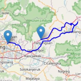
14_1denotes the first part of the dataset gathered on the 14th day of telemetry capture. - vehicle_map_14_1: High-resolution route map of the test vehicle's trip for gathering telemetry.
| id | timestamp | vehicle_id | latitude | longitude | altitude | speed | rpm | engine_temp | throttle_pos | engine_load | fuel_level | fl_press | fl_temp | fl_bat | fr_press | fr_temp | fr_bat | rl_press | rl_temp | rl_bat | rr_press | rr_temp | rr_bat |
|---|---|---|---|---|---|---|---|---|---|---|---|---|---|---|---|---|---|---|---|---|---|---|---|
| 44 | 2025-11-07 04:15:27+00 | -6.972864 | 107.6471638 | 698.3 | 0 | 699 | 84 | 15.68627 | 29.80392 | ||||||||||||||
| 45 | 2025-11-07 04:15:36+00 | -6.972861 | 107.6471588 | 698.9 | 0 | 698 | 84 | 15.29412 | 29.80392 | ||||||||||||||
| 46 | 2025-11-07 04:15:41+00 | -6.972859 | 107.6471562 | 699.0 | 0 | 711 | 85 | 15.29412 | 29.01961 | ||||||||||||||
| 47 | 2025-11-07 04:15:46+00 | -6.972858 | 107.6471558 | 699.4 | 0 | 709 | 85 | 15.68627 | 29.01961 | ||||||||||||||
| 48 | 2025-11-07 04:15:51+00 | -6.972857833 | 107.6471568 | 699.6 | 0 | 711 | 85 | 15.68627 | 28.62745 |
| timestamp | latitude | longitude | altitude | speed | engine_load | fl_pressure | fl_temp | fr_pressure | fr_temp | rl_pressure | rl_temp | rr_pressure | rr_temp | dist_m | sum_dist_m | elev_m | tr_fl | tr_fr | tr_rl | tr_rr |
|---|---|---|---|---|---|---|---|---|---|---|---|---|---|---|---|---|---|---|---|---|
| 2025-11-14 05:33:57+00 | -6.908889667 | 107.6577782 | 717.2 | 3 | 60.0 | 27.41117 | 35.0 | 28.86149 | 35.0 | 29.58666 | 35.0 | 24.22045 | 34.0 | 1.5482 | 1.5482 | 0.1000 | 5.97e-07 | 1.53e-06 | 2.15e-06 | 1.44e-06 |
| 2025-11-14 05:34:02+00 | -6.908884667 | 107.6578010 | 717.5 | 1 | 81.56863 | 27.41117 | 35.0 | 28.86149 | 35.0 | 29.58666 | 35.0 | 24.22045 | 34.0 | 2.5775 | 4.1257 | 0.3000 | 5.97e-07 | 1.53e-06 | 2.15e-06 | 1.44e-06 |
| 2025-11-14 05:34:07+00 | -6.908887000 | 107.6578203 | 718.2 | 1 | 62.35294 | 27.41117 | 35.0 | 28.86149 | 35.0 | 29.58666 | 35.0 | 24.22045 | 34.0 | 2.1462 | 6.2719 | 0.7000 | 5.97e-07 | 1.53e-06 | 2.15e-06 | 1.44e-06 |
| 2025-11-14 05:34:12+00 | -6.908886833 | 107.6578295 | 719.1 | 1 | 59.60784 | 27.41117 | 35.0 | 28.86149 | 35.0 | 29.58666 | 35.0 | 24.22045 | 34.0 | 1.0157 | 7.2877 | 0.9000 | 5.97e-07 | 1.53e-06 | 2.15e-06 | 1.44e-06 |
| 2025-11-14 05:34:17+00 | -6.908890833 | 107.6578455 | 719.5 | 1 | 84.70588 | 27.41117 | 35.0 | 28.86149 | 35.0 | 29.58666 | 35.0 | 24.22045 | 34.0 | 1.8213 | 9.1090 | 0.4000 | 5.97e-07 | 1.53e-06 | 2.15e-06 | 1.44e-06 |
NASA C-MAPSS Dataset
Download ZIP (12.4 MB)This benchmark dataset contains simulated run-to-failure trajectories of aircraft turbofan engines generated using NASA's Commercial Modular Aero-Propulsion System Simulation (C-MAPSS) tool. It is widely used to evaluate Remaining Useful Life (RUL) predictions.
- train_FD001.csv: Run-to-failure sensor histories for 100 engines (operating under sea-level conditions with high-pressure compressor degradation).
- test_FD001.csv: Operational histories for 100 test engines where recording is truncated prior to failure.
- RUL_FD001.csv: Ground-truth Remaining Useful Life (remaining cycles) for the 100 test engines.
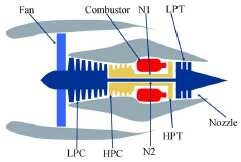
As detailed in the accompanying "Damage Propagation Modeling.pdf" and "readme.txt", each turbofan simulation begins with normal operations and develops varying degrees of initial wear and manufacturing deviations (unknown to the model). Over operational cycles, component faults propagate (such as High-Pressure Compressor blade erosion and Fan blade wear) until critical failure. The data is contaminated with sensor noise and consists of 26 columns: Engine ID, cycles, 3 operational settings, and 21 distinct thermo-mechanical sensors.
| unit_number | time_in_cycles | op_setting_1 | op_setting_2 | op_setting_3 | sensor_1 | sensor_2 | sensor_3 | sensor_4 | sensor_5 | sensor_6 | sensor_7 | sensor_8 | sensor_9 | sensor_10 | sensor_11 | sensor_12 | sensor_13 | sensor_14 | sensor_15 | sensor_16 | sensor_17 | sensor_18 | sensor_19 | sensor_20 | sensor_21 |
|---|---|---|---|---|---|---|---|---|---|---|---|---|---|---|---|---|---|---|---|---|---|---|---|---|---|
| 1 | 1 | -0.0007 | -0.0004 | 100.0 | 518.67 | 641.82 | 1589.70 | 1400.60 | 14.62 | 21.61 | 554.36 | 2388.06 | 9046.19 | 1.30 | 47.47 | 521.66 | 2388.02 | 8138.62 | 8.4195 | 0.03 | 392 | 2388 | 100.00 | 39.06 | 23.4190 |
| 1 | 2 | 0.0019 | -0.0003 | 100.0 | 518.67 | 642.15 | 1591.82 | 1403.14 | 14.62 | 21.61 | 553.75 | 2388.04 | 9044.07 | 1.30 | 47.49 | 522.28 | 2388.07 | 8131.49 | 8.4318 | 0.03 | 392 | 2388 | 100.00 | 39.00 | 23.4236 |
| 1 | 3 | -0.0043 | 0.0003 | 100.0 | 518.67 | 642.35 | 1587.99 | 1404.20 | 14.62 | 21.61 | 554.26 | 2388.08 | 9052.94 | 1.30 | 47.27 | 522.42 | 2388.03 | 8133.23 | 8.4178 | 0.03 | 390 | 2388 | 100.00 | 38.95 | 23.3442 |
| 1 | 4 | 0.0007 | 0.0000 | 100.0 | 518.67 | 642.35 | 1582.79 | 1401.87 | 14.62 | 21.61 | 554.45 | 2388.11 | 9049.48 | 1.30 | 47.13 | 522.86 | 2388.08 | 8133.83 | 8.3682 | 0.03 | 392 | 2388 | 100.00 | 38.88 | 23.3739 |
| 1 | 5 | -0.0019 | -0.0002 | 100.0 | 518.67 | 642.37 | 1582.85 | 1406.22 | 14.62 | 21.61 | 554.00 | 2388.06 | 9055.15 | 1.30 | 47.28 | 522.19 | 2388.04 | 8133.80 | 8.4294 | 0.03 | 393 | 2388 | 100.00 | 38.90 | 23.4044 |
Reproducibility Note
All code notebooks were developed on Google Colab linked to Google Drive storage. To run them locally, ensure you install dependencies using `pip install -r requirements.txt` (including `lifelines`, `xgboost`, and `lightgbm`), adjust G-Drive mounting lines, and re-map CSV paths relative to your local root directory.
Explore the Codebase
Access the complete machine learning models, lifelines survival analysis regressions, ESP32-S3 microcontroller firmware, and turbofan/tire telemetry preparation pipelines on GitHub.